How To View All Data Plot In Matlab

iv. Arrays

Plotting Graphs

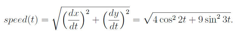
In this section we will use MATLAB 'south plot command to produce graphs. In Sections 6and 8 you will run into in that location are two other commands to create graphs, namely fplot which uses function Grand-files and ezplot which is within the Symbolic Math Toolbox.

If x = {x(1), ten(2), . . . , x(n )} and y = {y(1), y(two), . . ., y(n)}, so the MATLAB control plot(ten,y) opens a graphics window, chosen a Figure window, scales the axes to fit the data, plots the points (x(1), y(1)), (10(2), y(2)), . . . , (x(due north), y(n)), and then graphs the data past connecting the points with straight lines. If a Figure window already exists, some other plot command clears the electric current Figure window by default (unless instructed not to do and then) and draws a new plot. Blazon in the following as an attempt to graph y = sinx for 0 ≤ ten ≤ 2π. [You lot could replace the terminal 2 lines with plot(x,sin(x)).]

articulate all

x=linspace(0,ii*pi,11);

y=sin(x);

plot(10,y)

Clearly this endeavor is unacceptable because we accept not used sufficient points!Change the 11 to 201 and execute the code again.

In general, most graphs can be satisfactorily plotted using arrays of, say, 101 to 201 points,although erratic or wildly fluctuating functions would require many more points. Please annotation that y'all only need two points to plot a single straight line. For example, to plot a straight line from the point (one,vii) to the point (three,-five) you demand the command plot([i iii],[7 -5]).

Note: Students often get this wrong by forgetting that the first array ever containsthe x-coordinates, not the two coordinates of the first indicate. Similarly, the second array contains the y-coordinates.

Do 1: Plot the graph of y =xex/ x^two − π² for −three ≤ x ≤ 2 using a footstep-size of 0.02. You will need three dots in the expression to generate the array y.

Practice 2: Plot the graph of y = sin9x + sin10.5x + sin12x for −π ≤ 10 ≤ π using 601points.

Plotting several graphs on the aforementioned axes

Example one: Suppose you lot want to plot the oscillations y1 = cost, y2 = cos3t and theirsum y3 = y1 + y2, for 0 ≤ t ≤ 4π, on the aforementioned axes. Here t is measured in seconds and y1, y2, y3 are measured in cm.

clear all

t=linspace(0,four*pi,201);

y1=cos(t); y2=cos(3*t); y3=y1+y2;

plot(t,y1,t,y2,t,y3)

You notice that nosotros found the 3 y-arrays in a single line of lawmaking and they were plotted in different colours. But the empty space at the right cease of the graphs is annoying, and how can nosotros label the output so that each graph can exist identified? There are many facilities provided past MATLAB to assist you lot in producing attractive, meaningful graphs. Change the above Grand-file to the following (this is of import!):

clear all

t=linspace(0,4*pi,201);

y1=cos(t); y2=cos(3*t); y3=y1+y2;

axis([0 iv*pi -2 two]) % specifies the axes limits

hold on

plot(t,y1,'b--',t,y2,'thou:',t,y3,'r')

legend('y1=cos(t)','y2=cos(3*t)','y3=y1+y2')

plot([0 4*pi],[0 0],'k') % adds the t axis in black

xlabel('time in seconds')

ylabel('deportation in cm')

championship('oscillations')

hold off

A curt diversion

To get assistance with the MATLAB commands featured to a higher place and in the next case,you can use the help facility. Enter each of the following subsequently the >> prompt and carefully read the information until you empathise precisely what each of the lines in the previous (or side by side) 1000-file is accomplishing.

assistance axis
help plot
help hold
assistance legend
assistance text
help impress a menu of print options for your Figure

Alternatively, if yous do non know the precise name of a MATLAB command for which youneed help, y'all can click on the Assistance button at the tiptop of the MATAB Command Window, then click on "MATLAB Help" followed by "MATLAB Functions Listed by Category" and and so on a topic of interest. For instance, to go help on many graphics related commands, click on Plotting and Information Visualization.

Another assist option is the lookfor facility. Suppose you were interested in commands involving the apply of circuitous numbers. After the >> prompt enter lookfor complex.

Example ii: By using hold on and agree off, yous can plot several functions on the aforementionedaxes using a number of plot commands. The functions f(10) = x2 and f−i(x) = √ x are inverse functions for x ≥ 0 and hence their graphs must exist reflections through the line y = ten. Execute the following One thousand-file, advisedly noting the results of each command:

articulate all % file bachelor in M-files folder as file1.m

centrality([0 four 0 4]), axis foursquare

concord on

x1=linspace(0,ii,101);

y1=x1.^two; % note the dot

plot(x1,y1)

x2=linspace(0,iv,101);

y2=sqrt(x2);

plot(x2,y2)

plot([0 4],[0 4],'grand:') % dotted line in black from (0,0) to (iv,iv)

text(1.v,iii.five,'y=x^2')

text(three.1,1.7,'y=sqrt(x)')

grid on % adds grid lines if you lot desire them

title('reflection holding of inverse functions')

Zoom on

MATLAB provides an interactive tool to expand sections of a plot to come across more than detail. Thisis specially useful if y'all need to obtain authentic information about where ii graphs intersect, or to find the coordinates of an farthermost signal. The command zoom on, either in your M-file or after the >> prompt turns on the zoom mode. And so go to the Figure window, place the arrow where you want an enlargement and click with the left button. Keep this process and yous tin zoom in to obtain iii or four decimal place accurateness.

graph

Example: Suppose y'all want to find graphically the point of intersection of y = tanx andy = 1− x3. (Note that there are other non-graphical ways of doing this, described in Sections half-dozen and 8.) Firstly, plot both of these functions on the aforementioned axes for −1.two ≤ x ≤ 1.ii, with at least 800 points to enable zooming. You lot might also like to add together the x and y axes to obtain a figure similar to that on the previous folio. Enter the command zoom on . Then zoom in at the signal of intersection until you are able to find its coordinates to the accuracy of (0.6376 , 0.7408).

Exercise: Plot y = 10e−t sin t for 0 ≤ t ≤ 2π and and then use zoom on to find its maximum 5alue.

Creating separate graphs in one M-file

If yous want ii dissever Figures to be created in i G-file, you tin employ the figure(northward)command where north is a number associated with the window and precedes the fix of plotting

commands.

Instance: At time t seconds, t ≥ 0, a moving point has coordinates x = sin2t, y = cos3t(metres), and and so its speed is given past

speed

Plot the path taken by the indicate over one wheel 0 ≤ t ≤ 2π, where t is regarded as aparameter, and likewise plot the speed against time. Employ the following M-file. (You can add your own labels, etc.)

clear all % file available in Thousand-files folder every bit file2.k

t=linspace(0,2*pi,500);

ten=sin(ii*t);

y=cos(iii*t);

figure(one)

plot(10,y)

axis equal % same scale (metres) on each axis

speed=sqrt(4*cos(2*t).^2+nine*sin(3*t).^2); % note the dots

figure(two)

axis([0 2*pi 0 4])

hold on

plot(t,speed)